Lab-trained. NASA-funded research intern. Ready for her first role in healthcare or biotech.
Curious how living things work, and how they came to be.
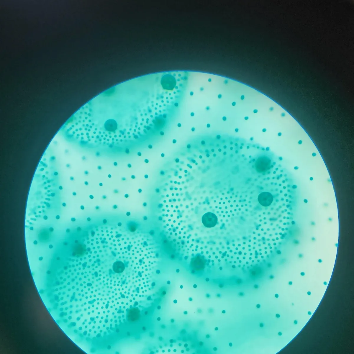
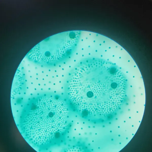
Volvox algae, photographed by Mia through her first microscope.
Scroll to look closer
0GPA, A.S. in Biology Prince George's Community College
0GPA, Eleanor Roosevelt High School
0Lab and modeling techniques trained on
0NASA-funded research internship, 2024
Seeing how beautiful and complicated life was even at a cellular level was eye-opening.
Mia, on her first microscope photos
Featured research · Feb to May 2024
Towards the end of degrading plastics.
A NASA-funded research internship at Prince George's Community College. The first time Mia worked on a problem that had no answer key.
Poster by Mia LaPlace and Christian Reyes, advised by Nadene Houser-Archield · tap to enlarge
01 · The problem
Plastics that won't break down.
Many plastics are built from long chains of polyvinyl alcohol. The goal: find a clean, effective way to change those chains so the plastic can be degraded or repurposed.
02 · The bench work
Oxidizing secondary alcohols.
Mia tested extraction, reflux and distillation to find the cleanest route from a secondary alcohol to its ketone, the first step toward the target reaction.
Extraction
Reflux
Distillation
03 · The model
Finding a transition state in 3D.
She trained in computational chemistry with GaussView 6.1, modeling a transition state for pentan-3-one to help develop the program.
04 · What it taught her
A failed run is still data.
"This experience has shown me what it's like to attempt solving a problem without a current solution." She wrote her own procedures, got creative with limited materials, and learned the persistence real experiments need.
The lab notebook
Open her notebook. Check her numbers.
Real experiments from her coursework, one course per tab. Every number comes from her own reports and was checked against her data.
BSCI423 · Principles of Immunology Laboratory · University of Maryland · Spring 2025 · 7 lab reports · group bench work, her own analysis and write-up
Controls
Standards, 1 to 0.0005 µg/ml
Patient serum
Lab 7 · ELISA
Measuring a lupus marker in patient serum.
An indirect ELISA for anti-DNA antibodies. Three kinds of negative control, twelve two-fold standards in triplicate, background subtraction, then a standard curve to read the unknown.
Her standard curvey = 0.334x + 0.0268
ELISA
Plate reader, 595 nm
Serial dilution
Standard curve
Lab 7 · ELISA · Spring 2025
Determining the concentration of anti-DNA antibodies in patient serum
The question
Anti-DNA antibodies are a marker for lupus. Is there a measurable amount in this patient sample?
What she did
Ran an indirect ELISA on a DNA-coated 96-well plate, read at 595 nm.
Built three negative controls: no antigen, no primary antibody, no secondary antibody.
Made a 12-step two-fold dilution of the antibody standard (1 down to 0.000488 µg/ml), in triplicate.
Subtracted background (0.0407), averaged the triplicates and fit a standard curve: y = 0.334x + 0.0268.
What she found
Anti-DNA antibody was detectable. The sample read between her 0.125 and 0.25 µg/ml standards (in-well). She also flagged three wells that went negative after background subtraction as a data-quality issue.
"While it is not enough for a diagnosis, the results of this ELISA could serve as an indicator of a potential autoimmune disease."
Plate readings were shared by her lab group. The analysis and report are her own.
Share of cells that divided after TLR9 stimulation
B cells50.5%
T cells9.7%
0%50%100%
Lab 9 · Flow cytometry
Which immune cells answer the call?
She labeled mouse spleen cells with CFSE dye, stimulated them, and used flow cytometry to see which cells divided. Her hypothesis: only B cells would respond. It held.
Flow cytometry
CFSE proliferation
Gating
Sterile cell culture
Lab 9 · Flow cytometry · Spring 2025
Measuring B and T lymphocyte proliferation via flow cytometry
The question
When spleen cells are stimulated through TLR9, do B cells, T cells, or both start dividing?
What she did
Labeled mouse spleen lymphocytes with CFSE, a dye that halves with every cell division.
Cultured the cells for two days at 37 °C in CO₂, under sterile technique.
Stained B cells (APC) and T cells (PE), then fixed them with paraformaldehyde.
Ran a six-tube control panel: unstained, isotype, PE only, APC only, CFSE only, and test.
Read histograms and quadrant plots and gated the dividing populations.
What she found
50.5% of B cells had divided, against 9.7% of T cells. Her hypothesis was supported: B cells responded to TLR9 and T cells mostly did not.
"The no-labeling control gave us the baseline of autofluorescence without any dyes or markers present."
Group lab. The analysis, interpretation and report are her own.
Labs 5-6 · Immunoprecipitation + Western blot
Pulling one protein out of a cell.
She isolated the ZAP-70 kinase from T-cell lysate, cast her own SDS-PAGE gel, ran a Western blot, and sized the signal from a standard curve. Then she questioned her own result.
Estimated size≈ 68.9 kDa
Immunoprecipitation
SDS-PAGE
Western blot
Bio-Rad ChemiDoc
Labs 5-6 · Protein biochemistry · Spring 2025
Detection and quantification of ZAP-70 via immunoprecipitation and Western blotting
The question
Can one specific signaling protein, ZAP-70, be pulled out of T cells and detected by size?
What she did
Lysed T cells and immunoprecipitated ZAP-70 with an antibody and Protein A agarose beads, with a beads-only control.
Hand-cast a discontinuous SDS-PAGE gel (separating and stacking layers) and denatured the samples.
Transferred to nitrocellulose, blocked, probed, and detected with ECL chemiluminescence on a Bio-Rad ChemiDoc.
Plotted log molecular weight against migration distance: y = -0.026x + 5.54.
What she found
The signal at 27 mm worked out to about 68.9 kDa, in the expected range for ZAP-70. She didn't stop there: the lane showed a smear rather than a clean band, so she flagged likely nonspecific binding, noted that overexposure ruled out band density, and proposed fixes.
"Column 5 did not appear as a band but as a large smudge, which is most likely not the ZAP 70, but nonspecific binding taking place."
Group lab of four. The analysis and report are her own.
Known 0.4 mg/ml
Unknown
AgglutinatedSettled (no reaction)
Lab 3 · Agglutination titration
Finding an unknown by halving.
Two-fold serial dilutions across a microtiter plate. The known antibody reacted through three wells, the unknown through two, so the unknown held about half the concentration.
Her estimate0.2 mg/ml
Serial dilution
Hemagglutination
Micropipetting
Lab 3 · Agglutination · Spring 2025
Determining antibody concentration using agglutination assays
What she did
Ran two-fold serial dilutions (50 µl transfers) of a rabbit anti-sheep red blood cell antibody across a round-bottom 96-well plate.
Compared a known 0.4 mg/ml standard against an unknown, in triplicate rows, after 24 hours.
What she found
The known sample agglutinated through column 3 and the unknown through column 2, one two-fold step less. Her estimate: 0.2 mg/ml. Two wells were borderline, so she checked the answer both with and without them.
"Whether these rows were both included or excluded, the resulting concentrations remained unchanged."
Also in this course: complement-mediated killing of E. coli (spread-plating, colony counts, percent-kill math), immunofluorescence microscopy of B-cell receptor internalization, and Ouchterlony double diffusion.
CHEM272 · General Bioanalytical Chemistry Laboratory · University of Maryland · Fall 2024 · 9 experiments · her own data, calculations and write-ups
Her BSA standard curve: absorbance vs. protein in the cuvette. Use the arrow keys to read each standard.
BSA standards (cuvette concentration, average absorbance ± SD)
µg/mL
Absorbance
0
0.0003 ± 0.0006
2.51
0.034 ± 0.004
6.26
0.107 ± 0.002
12.5
0.318 ± 0.004
25.1
0.60 ± 0.01
37.6
0.77 ± 0.03
50.1
1.01 ± 0.01
Experiment 2 · Protein quantitation
What's in the mystery drink?
She built a seven-point protein standard curve by UV-Vis spectrophotometry, measured a diluted unknown in triplicate, worked back through a 1:4000 dilution, and matched it to the closest candidate: 2% milk.
Fit qualityR² = 0.9882
UV-Vis spectrophotometry
Beer's Law
Serial dilution
Excel LINEST
Error propagation
Experiment 2 · CHEM272 · Fall 2024
Protein quantitation of an unknown by Beer's Law
The question
An unknown drink is one of three: protein-enriched milk, a protein shake, or 2% milk. Which one is it?
What she did
Diluted a 0.501 mg/mL BSA stock into seven standards with a P-1000 micropipette.
Added Pierce protein reagent, blanked the spectrophotometer on reagent + water, and read each standard in triplicate.
Fit the standard curve (y = 0.0206x + 0.0117, R² = 0.9882) and used LINEST for the uncertainty: ε = 0.021 ± 0.001 mL µg⁻¹ cm⁻¹.
Measured the unknown (absorbance 0.150 ± 0.001), then scaled through three dilutions (1:4000 total).
What she found
The unknown held 28,000 ± 400 µg/mL of protein. The closest candidate was 2% milk.
Protein-enriched milk85,000
Protein shake71,000
2% milk38,000
Her unknown28,000 ± 400
µg/mL of protein
"The percentage error is the smallest between the unknown and the 2% milk (26% error) compared to the others (67% and 61% error)."
The pKa values she measured, by unknown. Use the arrow keys to read each value.
Experiment 6 · Titration
Is this supplement safe for PKU patients?
Written as a memo to a supervisor. She standardized her base against a primary standard, titrated three unknown amino acids, and identified them from their pKa values.
IdentifiedLeucine · Histidine · Glutamate
Acid-base titration
KHP standardization
First-derivative plots
pKa analysis
Experiment 6 · CHEM272 · Fall 2024
Identifying amino acids by titration: a safety memo
The scenario
A supplement company needs to know whether its product contains phenylalanine, which people with phenylketonuria (PKU) must avoid.
What she did
Standardized NaOH against potassium hydrogen phthalate: 0.2426 ± 0.0006 M.
Titrated three unknown amino acids with a pH probe and built first-derivative plots to find each equivalence point.
Read pKa values at the half-equivalence points and matched them to literature values.
What she found
Unknown A (pKa 2.49, 9.63) was leucine. Unknown B (1.88, 6.13, 9.31) was histidine. Unknown C (2.26, 4.40, 9.76) was glutamate. No phenylalanine, so the supplement should be safe for PKU patients, with more testing recommended. She also rejected a tempting wrong match:
"While Unknown B has the lowest percentage error of 4.70% with Phenylalanine, Unknown B is triprotic and Phenylalanine is diprotic, so it is very unlikely."
Active drug by mass, acetylsalicylic acid
Bayer66.8%
Knock-off60.5%
0%50%100%
Experiment 8 · Drug assay
Catching a weaker counterfeit.
She titrated pure aspirin, Bayer, and an online knock-off, then worked out each one's pKa, the drug's molecular weight, and how much active drug each tablet really held.
pH titration
Reference standard
Mass-percent assay
Experiment 8 · CHEM272 · Fall 2024
Counterfeit aspirin analysis by pH titration
What she did
Dissolved pure acetylsalicylic acid, a Bayer tablet and an internet knock-off, and titrated each with 0.1 M NaOH while tracking pH.
Found each pKa by half-equivalence interpolation: pure 5.99, Bayer 5.97, knock-off 6.47.
Calculated the drug's molecular weight from the titration: 188.18 g/mol against the literature 180.16.
What she found
Bayer held 66.8% active drug by mass. The knock-off held 60.5%. She tied the result back to the patient: a weaker tablet means taking more of it to get the same effect as one real dose.
Keq0.0066± 0.0003, triplicate
Experiment 4 · Enzyme equilibrium
Watching an enzyme reach balance.
She followed alcohol dehydrogenase turning NAD⁺ into NADH at 342 nm for 30 minutes, calculated the equilibrium constant under three conditions, and tested Le Chatelier's principle with an extra spike of NAD⁺.
Enzyme assay
UV monitoring, 342 nm
ICE tables
Also in this course: glassware accuracy and precision (her best method: 0.996 ± 0.002 g/mL, 0.119% error), reaction kinetics and model fitting by R², Tris buffers and Henderson-Hasselbalch, iodometric titration of vitamin C, and electrochemistry with the Nernst equation.
BSCI335 · Mammalogy lab · University of Maryland · Spring 2026 · lab worksheets she completed: behavior, skulls, limbs, reproduction, phylogenies
Share of on-screen time spent feeding, from the 21 behavior bouts she timed. The rest was spent watching for danger.
Cow62%
Horse97%
Deer34%
Squirrel23%
0%50%100%
Largest animal at top, smallest at bottom, in the order she graphed them.
Lab 6 · Animal behavior
Do bigger animals worry less?
She built an ethogram (a catalog of behaviors), wrote a testable hypothesis, and timed every switch between feeding and watching in field videos of four species. She also identified wild mammals in Smithsonian camera-trap footage from Panama.
Her conclusion"The data partially supported my hypothesis."
Ethograms
Focal-animal sampling
Camera-trap ID
Excel graphing
Lab 6 · BSCI335 Mammalogy · Spring 2026
Observing and quantifying behavior
The question
Is there a relationship between an animal's body size and how it splits its time between feeding and watching for danger?
What she did
Identified two mammals caught on Smithsonian camera traps on islands in the Panama Canal: an opossum (her best match, a Central American woolly opossum) and a tayra (Eira barbara), a member of the weasel family. She checked which species live in the region before settling on each.
Built a partial ethogram of feeding and vigilance postures for squirrels, marmots, deer, cows and horses.
Hypothesis: as body size increases, time spent vigilant goes down and time spent feeding goes up. Her proposed mechanism: predation risk, since smaller animals are more likely to be eaten.
Chose continuous focal-animal sampling over scan sampling, and logged 21 timed bouts in field clips from the Rocky Mountain Biological Laboratory.
Graphed time spent feeding against time spent watching, for all four species, in Excel.
What she found
The horse fed for 97% of its time on screen and the cow for 62%. The deer (34%) and the ground squirrel (23%) spent most of their time watching. The pattern followed body size overall, though not exactly.
"The data partially supported my hypothesis."
Percentages are worked out from the bout times in her data table. Parts of this lab were done with a partner; the report is her own.
Forelimb length divided by hind-limb length, from her measurements. Use the arrow keys to read each species.
Forelimb to hind-limb length ratio
Species
Ratio
Frog
0.42
Rabbit
0.53
Cat
0.70
Mole
0.77
Human
0.79
Horse
0.82
Chimpanzee
1.13
Bat
2.84
Limbs & locomotion · Measurement
Reading lifestyle from bones.
She measured ten limb bones for each of eight species, from frog to bat, with units on every column. Then she turned them into ratios so animals of different sizes compare fairly, and ranked them.
From 80 bone measurements40 ratios
Specimen measurement
Ratio analysis
Form and function
Limbs & Locomotion · BSCI335 Mammalogy · Spring 2026
What limb proportions say about how an animal moves
What she did
Measured the humerus, radius, carpals, metacarpals, phalanges, femur, tibia, tarsals, metatarsals and toe bones of a frog, rabbit, human, cat, bat, chimpanzee, horse and mole.
Calculated five ratios per species, including forelimb length over hind-limb length.
Classified limb posture: cat digitigrade (on its toes), chimpanzee plantigrade (flat-footed), horse unguligrade (on hooves).
Predicted where species she didn't measure would fall: a kangaroo near the frog and rabbit, a spider monkey near the chimpanzee.
What she found
The forelimb-to-hind-limb ratio runs from 0.42 in the leaping frog to 2.84 in the bat. The bat's hand bones are 3.67 times the length of its upper arm, the highest ratio in her table. Her 40 ratios check out against her raw measurements, to within rounding.
"It is important to use ratios because animals vary in size, but their actual proportions may be similar or different."
Her recorded path through the key for skull 1. Each dot is one either/or choice.
Comparative skulls · Dichotomous keys
Six unknown skulls, one key.
Using the lab manual's keys, she worked each unknown skull through a chain of either/or choices, keyed all six to order and the carnivores and rodent to family, and wrote down every step.
Compared skulls across carnivores, marsupials, primates and hoofed mammals, noting the features each group shares.
Wrote dental formulas: 30 teeth for the cat, 50 for the Virginia opossum.
Read diet from teeth: selenodont molars in the deer, bunodont in the pig, and sharper molars in the coyote than in the raccoon.
Keyed six unknown skulls with the lab manual's dichotomous keys, recording the full couplet path for each.
Her determinations
Skulls 1 and 6: Carnivora, dog family (Canidae). Skull 2: Rodentia, squirrel family (Sciuridae). Skull 3: Carnivora, raccoon family (Procyonidae). Skull 4: Artiodactyla, the even-toed hoofed mammals. Skull 5: Lagomorpha, rabbits and hares.
"The coyote is sharper and indicates a carnivorous diet while the raccoon is duller, indicative of a more omnivorous diet."
Two divergence dates she looked up in TimeTree
Lab 7 · Phylogenetics
A family tree from protein code.
She aligned cytochrome b protein sequences from 51 mammals in the MEGA software, built a maximum-likelihood tree, then weighed her one-gene tree against a published study that used 6,845 genes.
Sequences aligned51 mammals
MEGA
Sequence alignment
Maximum likelihood
TimeTree
Lab 7 · BSCI335 Mammalogy · Spring 2026
Building a mammal phylogeny
What she did
Looked up divergence dates in TimeTree: about 94 million years since humans and bottlenose dolphins shared an ancestor, and about 180 million for gray squirrels and platypuses.
Traced one estimate back to a primary study and identified its question: are marsupials more closely related to monotremes than to placental mammals?
Aligned cytochrome b protein sequences for 51 mammals in MEGA and built a maximum-likelihood tree.
Read her tree: the domestic cat's closest wild relative in the dataset is the wildcat (Felis silvestris), and the domestic camelids form a paraphyletic group.
What she found
Her one-gene tree placed the hippo next to the horse, which conflicts with a published genome-wide tree built from 6,845 coding sequences (Tsagkogeorga et al., 2015). She judged the published tree more accurate because it drew on far more data.
"Highly related because they spent most of their evolutionary time together as a common ancestor and had less time to develop differences."
Also in this course: skull measurements and dental formulas across four mammal groups, and a reproduction lab with microscope slides, preserved specimens and labeled scientific drawings.
BIOM301 · Introduction to Biometrics · University of Maryland · 2026 · 11 modules of written analyses and worksheets, from descriptive statistics to chi-square
Chicken length vs. weight, 20 birds. Use the arrow keys to read each bird.Daylight vs. wheat height, 25 plants
Module 3 · Correlation
Telling a real pattern from noise.
She entered two datasets into Excel and computed Pearson's correlation. For the chickens she found a strong positive relationship. For the wheat she recognized the opposite: a weak relationship not worth leaning on.
Chicken length vs. weight, her Excel resultr = 0.97
Pearson's r
Scatter plots
Excel
Descriptive statistics
Module 3 · BIOM301 · 2026
Correlation: when a relationship is real
What she did
Entered length and weight for 20 chickens, and daylight exposure and height for 25 wheat plants, into an Excel workbook.
Computed Pearson's correlation coefficient and read both scatter plots.
Separately cautioned against extrapolating past the data and against treating correlation as cause.
What she found
Chickens: r = 0.97, a strong positive relationship. Wheat: she judged the coefficient of determination small, meaning daylight explained little of the variation in height.
"There is a positive correlation between length and weight of the chickens, as the chickens grow in length, the weight tends to increase."
Also in her workbook
Descriptive statistics for a 20-bird sample of weights: mean 35.4 g, median 35.0 g, standard deviation 18.0 g. All of them check out against her data.
Where her t = 8.65 falls on the t distribution (df = 38)
Module 10 · Two-sample t-test
Two training programs, one clear answer.
Genetically identical mice trained on Program A or Program B. She recognized two independent groups, set up the hypotheses, and chose a two-sample t-test. The difference in muscle strength was far too big to be chance.
Her write-upt = 8.65, df = 38, p < 0.001
Two-sample t-test
Paired vs. unpaired design
Hypothesis testing
Module 10 · BIOM301 · 2026
Matching the test to the design
The question, in her words
"Is there a significant difference between the mean muscle strength of all genetically identical mice using one training program versus another?"
What she did
Classified the study as unpaired: two independent groups of mice.
Stated the null hypothesis (no difference in mean strength between programs) and a two-sided alternative.
Reported a two-sample t-test and wrote the conclusion with its full statistical evidence.
In the same module, identified a headphones-and-reading study as paired and used a paired t-test.
What she found
"There is strong statistical evidence that the mean muscle strength differs between mice trained with Program A and Program B"
The scenario came from the course. The design calls and write-up are hers.
Truly safeTruly at riskWe decide "safe"CorrectType II errorSpecies left to declineThe one she guards againstWe decide "at risk"Type I errorMoney spent on a species that didn't need itCorrect
Module 8 · Type I vs. Type II errors
Choosing which mistake to risk.
An endangered species study: is the population big enough to last 100 years? She spelled out what each kind of error would cost in real terms, then made the call a conservation biologist would.
In her words"I would rather waste money and resources trying to help a species that didn't need it rather than potentially neglect a species into extinction."
Type I & II errors
Statistical judgment
Conservation
χ² test of independence8.33df = 1 · p = 0.004 · n = 200
Module 11 · Chi-square
Does the tea make a difference?
A dataset of 200 adults who sleep badly at least three nights a week, drinking chamomile or a control tea. Her chi-square test showed that whether sleep improved depended on which tea people drank.
Her decisionReject independence (p = 0.004)
Chi-square independence
Goodness-of-fit
Expected counts
Also in this course: probability and the binomial distribution, the normal distribution and z-scores, the Central Limit Theorem and standard error, confidence intervals for means and proportions, one-sample z- and t-tests, and experimental design (randomization, blocking and paired designs).
PHYS131 + PHYS132 · Fundamentals of Physics for Life Sciences I and II · University of Maryland · from Spring 2025 · lab reports co-authored in teams of four
How it works: a standing sound wave herds the beads into evenly spaced lines.
Bead-line spacing against 1 / frequency. Use the arrow keys to read each frequency.
Acoustic trap line spacing by frequency
Frequency
Spacing
1.8 MHz
403.3 µm
2.0 MHz
356.4 µm
2.26 MHz
313.1 µm
2.4 MHz
298.6 µm
Lab 9.1 · Acoustic trapping
Moving cells with sound.
The team drove a piezoelectric plate with a signal generator to set up an ultrasound standing wave in water, trapped 5-micron beads standing in for cells, and derived a model for the spacing between bead lines. Fitting their data gave the speed of sound in water.
Their measurement vs. the reference value1,516 vs. 1,496 m/s, about 1.3% apart
Signal generator
Piezo transducer
Model building
Linear fit
Lab 9.1 · PHYS132
Acoustic trapping with ultrasound
Why it matters
Ultrasound is best known for imaging, but it can also push on cells without touching them.
What they did
Built the model first: beads collect at the nodes of the standing wave, which sit half a wavelength apart, so the spacing is d = v / 2f.
Drove a piezoelectric plate at MHz frequencies to make a standing wave in a water chamber on the microscope stage, then added 5-micron silica beads.
Recorded the bead pattern at 1.8, 2.0, 2.26 and 2.4 MHz and converted pixels to meters (1.85 µm per pixel).
Plotted spacing against 1 / frequency. The slope, 758 m/s, is half the speed of sound.
What they found
Speed of sound in water: 1,516 m/s, against a reference of 1,496 m/s at 25 °C, about 1.3% apart. The sharpest bead pattern came near 2.4 MHz, their estimate of the device's resonance.
"One key application is the ability to apply forces to cells without direct contact."
Group lab, report co-authored by a team of four including Mia.
Average speed in µm/s, from microscope video
Neutrophils17
E. coli7.9
01020 µm/s
E. coli tracked by her group; neutrophils from class data.
Lab 1 · Cell tracking
Does this wound need antibiotics?
The team tracked bacteria and immune cells frame by frame in ImageJ. When the software's velocity readout came out wrong, they recomputed every velocity from the raw positions. The verdict: the patient's immune cells outpace the bacteria.
Their callNo antibiotics needed
ImageJ tracking
Microscope video
Unit calibration
Lab 1 · PHYS131 · February 2025
Wound healing and bacterial motion
The question
A patient's wound is infected with E. coli. Are the immune cells fast enough to handle it, or are antibiotics needed?
What they did
Tracked six E. coli cells and six wound-healing cells in microscope videos with ImageJ's Manual Tracking tool.
Converted pixels to micrometers, then recomputed velocities from the raw x and y positions with the distance formula when ImageJ's own velocity values were wrong.
Compared their averages with other groups' results and discussed the uncertainty from the spread of individual cell speeds.
What they found
Their E. coli averaged 7.9 µm/s, inside the class range of 3.2 to 22 µm/s. Class data put neutrophils at 17 µm/s, so the immune response should outpace the bacteria without antibiotics.
"The patient's neutrophils are moving much faster than the E. coli bacteria. Therefore, the neutrophils should heal the E. coli infected wound by themselves."
Group lab, report co-authored by a team of four including Mia.
A passive signal fading along an axon
Lab 8 · Nerve signaling
Why nerves can't just leak a signal.
The team modeled an axon as a chain of resistors, fit the voltage decay, and found a length constant of 1.51 mm. Over the meter from toe to spine, a passive signal would all but vanish, which is why nerves need action potentials.
Fitted length constant1.51 mm
Circuit modeling
Exponential fit
Neurophysiology
Lab 8 · PHYS132
Signal transmission along nerve axons
The question
Could a signal from an injured toe reach the spine by passive electrical spread alone?
What they did
Modeled the axon as repeating segments of resistors and a battery, treating the fluid outside the cell as a near-perfect conductor.
Calculated resistances for a 1 mm segment from R = ρL/A: 12.7 MΩ along the axon and 31.8 MΩ across the membrane.
Fit an exponential decay to voltage against distance and extracted a length constant of 1.51 mm.
Worked out how adaptations change it: doubling the diameter stretches the length constant by √2; 100 times the membrane resistance stretches it 10 times.
What they found
A meter of axon is about 662 length constants, so only e−662 of the signal would survive, effectively nothing. Passive spread fails over long distances.
"This suggests that the signal would be completely gone long before it reaches the spine and that your brain would never be informed of an injury to your toe using passive transport."
Group lab, report co-authored by a team of four including Mia.
Emission peak≈ 670 nmthe red glow of chlorophyll-a
400550700 nm
Lab 11 · Fluorescence spectroscopy
Making chlorophyll glow.
The team excited a chlorophyll solution with UV, white and colored light and read its fluorescence with a fiber-optic spectrometer set at 90° to the light path, so the source light stayed out of the reading. UV gave the cleanest peak.
Fluorescence
Spectrometer
Experimental controls
Also in these courses: Brownian motion of silica beads (and an honest call that the results were inconclusive), fluid flow through series and parallel channels, electric forces on charged microspheres, sound and hearing, and ray optics.
BIO-2010 · Microbiology · Spring 2024 · mixed-unknown identification, run online: she read Gram-stain and agar images, ordered her own follow-up tests, and interpreted the results
Each student gets a "patient" specimen holding two organisms. From the Gram stains and selective agars, Mia chose which tests to order in two rounds, up to six per organism, and narrowed each one down to a species.
Her identificationsS. pneumoniae · S. enterica
Gram stain interpretation
Selective & differential media
Biochemical tests
Clinical ID workflow
The lab bench
Trained hands. Twenty techniques.
Learned across her biology, chemistry, physics and statistics coursework and her internship. Tap any card for the plain-English version.
Also trained in lab safety, emergency procedures, proper handling of scientific equipment, and data keeping and analysis.
Under the lens
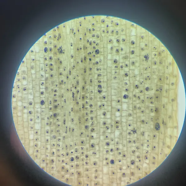
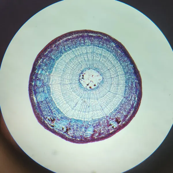
Her first look at life at the cellular level.
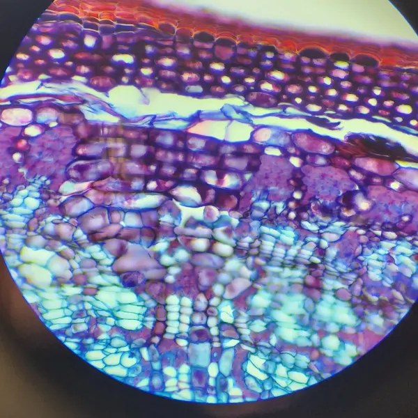
Taken in her Principles of Ecology and Evolution lab, freshman year. Move across a photo to magnify it.
Volvox algaeGreen algae that live as spinning colonies.
Onion rootRows of cells, some caught mid-division.
BasswoodA stem cross-section, growth rings and all.
Basswood, closerThe same stem at higher magnification.
Research proposal
Science communication · UMD BSCI423 · May 2025
Can the vaccine keep up with the virus?
"Moderna KP.2 Vaccine-Induced Immunity Against Emerging COVID-19 Spike Variants"
In her Principles of Immunology Laboratory course, Mia's team of four wrote a funding proposal to study how well the COVID-19 vaccine of the time protected against mutating strains, then presented it to the class. It was graded as if it were real.
Study design, timeline and materials list
How data would be measured and shown to the public
Turning deep science into plain language
Team writing and a live presentation
Education
Three schools. One direction.
Now
University of Maryland
Bachelor of Science, General Biology · College Park, MD
Principles of Immunology Lab
Bioanalytical Chemistry Lab
Mammalogy
Introduction to Biometrics
Physics for Life Sciences I & II
Research proposal writing
2024
Prince George's Community College
Associate of Science, Biology concentration · 3.84 GPA
Organic Chemistry II
Anatomy & Physiology
Evolution, Ecology & Behavior
Cellular & Molecular Biology
Environmental Biology
Calculus
2021
Eleanor Roosevelt High School
High school diploma · Greenbelt, MD · 3.98 GPA
AP Biology
AP Chemistry
AP Physics
Genetics
Environmental Science
Statistics
Beyond the lab
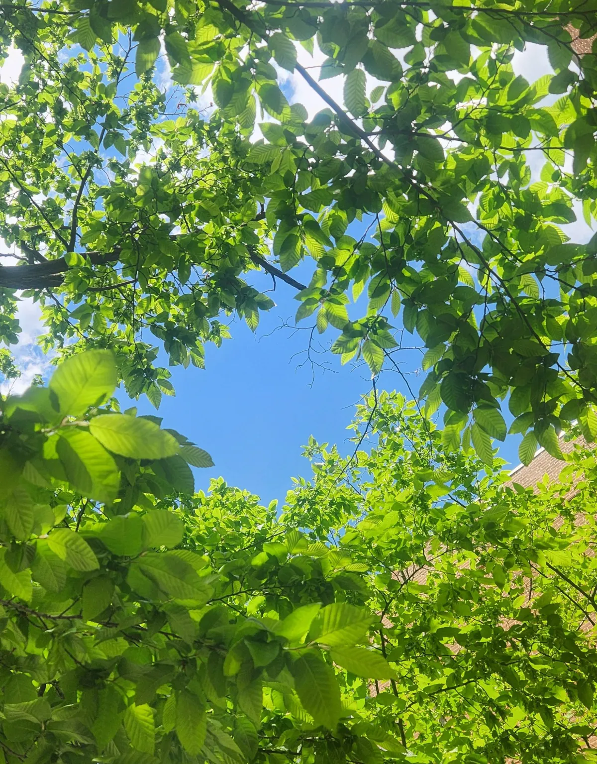
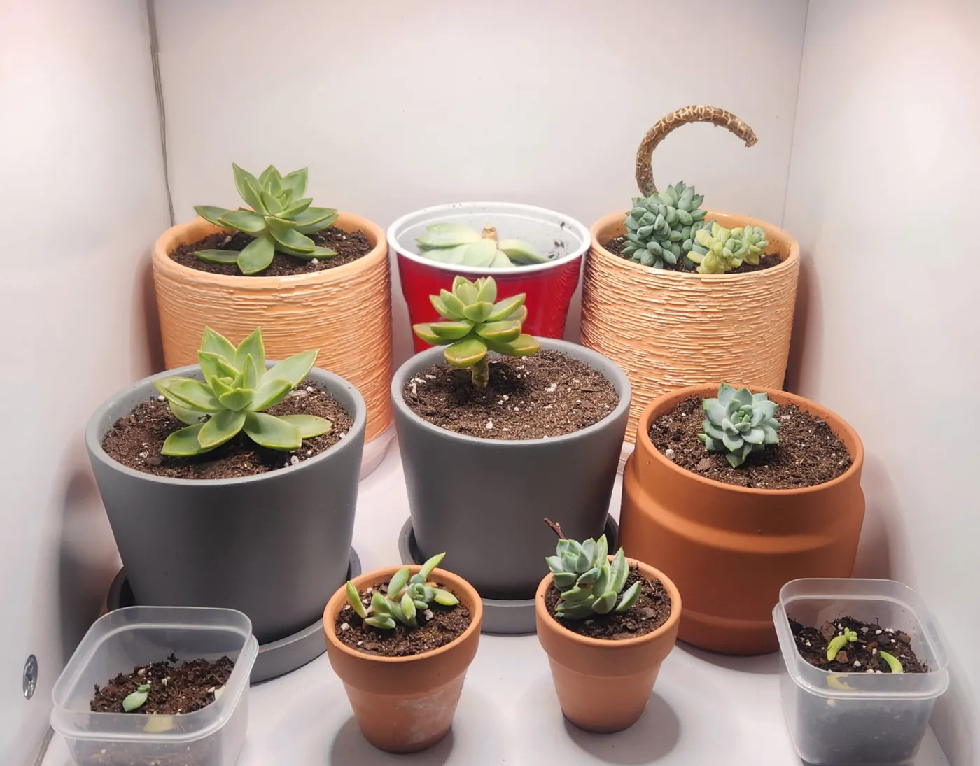
Every photo here is hers.
A science and nature enthusiast who loves explaining how the world works, to anyone who asks. Kids with silly questions included.
Looking up
Say hello. A short welcome from Mia.
The succulent shelf
How she works
Reliable
Detail-oriented
Patient
Team player
Active listener
Hardworking
Volunteer
Army Ten-Miler
Arlington, VA · October 2018. Early lessons in time management, teamwork and leadership.
Now hiring? Look closer.
Let's talk.
Mia is looking for her first full-time role in healthcare, biotechnology, or a research lab. She'd love to hear from you.